

To address the inventory management challenges, we employed MILP and DES. Both methods offer advantages in problem integration by combining the MILP with lateral transshipment. Because of the computational difficulty, simulations are the preferred approach. The discrete operation of the inventory in a simulation facilitated the incorporation of aspects of this method. Our research methodology was structured into two distinct phases. The first stage involved designing a mathematical inventory management model that minimized costs under uncertain demand conditions. The second stage focused on analyzing the lateral transshipment policy through simulations that replicated the same environmental conditions and included lateral transshipment variables.
Mixed integer linear programming
The parameters and decision variables used in MILP are shown in the following Tables 12 and 13:
In our model, time slots T represent the hospital’s operating hours, spanning n hours over k days, resulting in \(|T| = |N|\cdot |K|\) when \(demand^h,t\sim \textitU(\mu ,\sigma )\). The reorder cost encompasses the per- vial usage and transshipment costs. In the case of lateral transshipment, the cost incurred is solely for transportation purposes. We regard profit as a social benefit that prevents the spread of epidemic diseases through vaccination. Each vaccine vial contained |I| doses, denoted by |I|. Let p, \(c_u\), and \(c_o\) represent the revenue per dose when vaccinated, cost per dose when not administered, and cost per dose for leftover vaccines, respectively. Here, p symbolizes the benefit, and \(c_u\) and \(c_o\) represent the penalties. The objective of this problem was to maximize the number of vaccinated people and minimize the number of unvaccinated individuals. Thus, it minimized the total costs incurred during vaccination. Therefore, the importance hierarchy was \(p > c_u \ge c_o\)54. Minimizing costs in this context equates to maximizing revenue. The initial inventory for each hospital \(init_h\) was measured in vials. Considering the vaccine appointment demands of two hospitals, \(h^+\) and \(h^-\), each with their respective means \((\mu _h^+)\) and standard deviations \((\sigma _h^+)\), we formulated a problem that incorporated lateral transshipment.
The specific objective and constraint expressions for this problem are as follows.
$$\beginaligned \text Min \quad&Cost_R + Cost_T + Cost_O + Cost_U – Profit + Cost_H \endaligned$$
(1)
$$\beginaligned \text s.t \quad&Profit = \sum _i \in I\sum _j \in J\sum _h \in H\sum _t \in T p x_ij^ht – \sum _j \in J\sum _h \in H\sum _t \in T cy_j^ht \endaligned$$
(2)
$$\beginaligned&Cost_R = \sum _i \in I\sum _j \in J\sum _h \in H\sum _t \in Tc_r R^h,t \endaligned$$
(3)
$$\beginaligned&Cost_T = \sum _i \in I\sum _j \in J\sum _h \in H\sum _t \in Tc_t TR_(h^-, h^+)^t \endaligned$$
(4)
$$\beginaligned&Cost_O = \sum _h \in H\sum _k \in Ko_ \endaligned$$
(5)
$$\beginaligned&Cost_U = \sum _h \in H\sum _t \in Tu_h,t \endaligned$$
(6)
$$\beginaligned&\sum _i \in I\sum _j \in J x_ij^ht + u_h,t = demand^h,t \quad \forall h \in H, t \in T \endaligned$$
(7)
$$\beginaligned&inv^ – \sum _j \in Jy_j^ = o_h,k \quad \forall h \in H, k \in K \endaligned$$
(8)
$$\beginaligned&\sum _i \in I x_ij^ht \le M y_j^ht \quad \forall j \in J, h \in H, t \in T \endaligned$$
(9)
$$\beginaligned&\sum _i \in I x_ij^ht \ge y_j^ht \quad \forall j \in J, h \in H, t \in T \endaligned$$
(10)
$$\beginaligned&TR_(h^+, h^-)^t \ge z_(h^+, h^-)^t \quad \forall j \in J, h \in H, t \in T \endaligned$$
(11)
$$\beginaligned&TR_(h^+, h^-)^t \le Mz_(h^+, h^-)^t \quad \forall j \in J, h \in H, t \in T \endaligned$$
(12)
$$\beginaligned&z_(h^+, h^-)^t-1 + z_(h^-, h^+)^t\le 1 \quad \forall h \in H, t \ge 1 \endaligned$$
(13)
$$\beginaligned&z_(h^-, h^+)^t-1 + z_(h^+, h^-)^t\le 1 \quad \forall h \in H, t \ge 1 \endaligned$$
(14)
$$\beginaligned&inv^h,1 = init_h + |I| \cdot \left( TR_(h^+, h^-)^1 – TR_(h^-, h^+)^1\right) – \sum _i \in I\sum _j \in Jx_ij^h1 \quad \forall i \in I, j \in J, h \in H \endaligned$$
(15)
$$\beginaligned&inv^h,2 = inv^h,1 + |I| \cdot \left( TR_(h^+, h^-)^2 – TR_(h^-, h^+)^2\right) – \sum _i \in I\sum _j \in Jx_ij^h2 \quad \forall i \in I, j \in J, h \in H \endaligned$$
(16)
$$\beginaligned inv^N = inv^h^+,k + |I| \cdot \left( R^h,k + TR_(h^+, h^-)^k – TR_(h^-, h^+)^N\right) – \sum _i \in I\sum _j \in Jx_ij^hk – o_N \quad \forall i \in I, j \in J, h \in H, k \in K \endaligned$$
(17)
$$\beginaligned inv^h,t = inv^h^+,t-1 + |I| \cdot \left( R^h,t-2 + TR_(h^+, h^-)^t – TR_(h^-, h^+)^t\right) – \sum _i \in I\sum _j \in Jx_ij^ht \quad \forall i \in I, j \in J, h \in H, t \ge 3 \endaligned$$
(18)
$$\beginaligned&|I| \cdot \sum _j \in Jy_j^ht \le inv^h,t, \quad \forall h \in H, t \in T \endaligned$$
(19)
$$\beginaligned&\sum _n \in 1,2 R^(k-1)+n = 0 ,\quad \forall h \in H , k \in K \endaligned$$
(20)
$$\beginaligned&x_ij^ht \in \0,1\, \quad \forall i \in I, j \in J, h \in H, t \in T \endaligned$$
(21)
$$\beginaligned&y_j^ht \in \0,1\, \quad \forall j \in J, h \in H, t \in T \endaligned$$
(22)
$$\beginaligned&z_(h^-, h^+)^t \in \0,1\, \quad \forall h\in H, t \in T \endaligned$$
(23)
$$\beginaligned&inv^h,t \in \mathbf Z^+ \cup \0\ \endaligned$$
(24)
$$\beginaligned&R^h,t \in \mathbf Z^+ \cup \0\ \endaligned$$
(25)
$$\beginaligned&TR_(h^-, h^+)^t \in \mathbf Z^+ \cup \0\ \endaligned$$
(26)
$$\beginaligned&o_h,t \in \mathbf Z^+ \cup \0\ \endaligned$$
(27)
$$\beginaligned&u_h,t \in \mathbf Z^+ \cup \0\ \endaligned$$
(28)
$$\beginaligned&Profit \ge 0 \endaligned$$
(29)
$$\beginaligned&Cost_R \ge 0 \endaligned$$
(30)
$$\beginaligned&Cost_T \ge 0 \endaligned$$
(31)
$$\beginaligned&Cost_O \ge 0 \endaligned$$
(32)
$$\beginaligned&Cost_U \ge 0 \endaligned$$
(33)
The objective function (1) in our model was designed to minimize the total vaccination cost over the period \(|T| = |N|\cdot |K|\). This function comprised several costs, including reordering, lateral transshipment, underage, overage, profit, and holding. To minimize costs, the objective function was formulated as the total cost subtracted from profit.
Constraints (2–6) describe the costs involved in the objective function. Profit was calculated as the total number of doses sold during the period minus the total cost associated with the vials used for vaccination. The cost per used vial, along with transportation costs, was included to represent the cost of reordering. \(Cost_T\) denotes the transportation cost of transported vials. \(Cost_O\) and \(Cost_U\) represent the costs per dose for overage and underage vaccines, respectively. Equation (7) addresses the underage dose that occurs if the demand of a hospital is lower than the number of doses administered, resulting in leftover doses. Constraint (8) defines the overage dose, which is the quantity of vaccine remaining at the end of the day, and is thus discarded. The calculations of the overage dose amount and associated costs are included here. Constraints (9) and (10) establish the relationship between the vial and dose. Through the binary variables x and y and a large number denoted by M, the model ensured that if any dose was used, the corresponding vial was considered open; if no dose was used, the vial count remained 0.
Constraints (11–14) establish the directional nature of lateral transshipment, indicating that it is unidirectional rather than bidirectional. Equations (15–18) depict the dynamics of the vaccine inventory over period T. For example, at \(t=1\) (the first hour of day 1), the vaccine inventory was reduced from its initial level by the scheduled doses plus vials sent to other hospitals and increased by vials received from other hospitals. At \(t=2\), the inventory from the previous hour was adjusted by subtracting the demand and adding the transported vials. Constraints (15–16) are delineated separately to accommodate the indexing notation for reorders.
Constraint (17) pertains to inventory updates for the final hour of the day. Alongside constraint (18), which addresses hours other than 1 and 2, these constraints account for the exclusion of vaccines opened in the last hour and overage vaccines that are required to be discarded. Constraint (18) updates the vaccine inventory for times t excluding 1 and 2, thus increasing the inventory by the vials ordered 2 h prior and those received from other hospitals and decreasing it by the vials transported and doses administered. Because the inventory is measured in doses, Constraint (19) specifies the quantity of vaccine vials in the hospital. Equation (20) relates to reordering, which requires 2 h, and stipulates that no orders can be placed after hour \(n-1\) each day. Constraints (21–33) define the settings and ensure the non-negativity of each decision variable.
Discrete event simulation with lateral transshipment policy
The potential complexity of daily problems that may not be solvable within the given time limit (3600 s) using MILP and DES was utilized for policy analysis. The simulation environment mirrored the mathematical formulation by incorporating a lateral transshipment policy. Both MILP and DES operated under the assumption that the demand for vaccine appointments at two hospitals, \(h^+\) and \(h^-\), followed a uniform distribution with respective means \((\mu _h^+, \mu _h^-)\) and standard deviations \((\sigma _h^+, \sigma _h^-)\). Further, it was considered that the same individuals attended appointments at consistent times. This study focused on reactive lateral transshipments. The lateral transshipment policy extended Banerjee’s TBA policy to accommodate the specific characteristics of vaccines46.
The DES process was structured into six distinct phases: appointment visits, detection of vaccine stockout, execution of lateral transshipment, renewal of vaccine stock, reorder decisions, and finality of the day’s operations. This approach provided a comprehensive understanding of the dynamics involved in vaccine distribution and management under various demand scenarios.
The parameters of the simulation are shown in Table 14, which contain the same meaning with the proposed MILP.
Step 1. Appointment visit
Patients with appointments, as determined using a uniform distribution model, arrive at the hospital.
Step 2. Detection of vaccine stockout
The vaccine inventory is calculated for each hospital after completing all appointments have been fulfilled.
$$\beginaligned EOH_h,t = {\left\ \beginarrayll init_h – demand^h,t, \quad \text if \quad t = 1 \\ OH_h,t-1 – demand^h,t, \quad \text if \quad t \ge 2 \endarray\right. \quad demand^h,t\sim \textitU(\mu _h,\sigma _h),\quad \forall h \in H \endaligned$$
(34)
If \(EOH_h,t\) across different hospitals is negative, the process moves to Step 3; otherwise, it proceeds to Step 4.
Step 3. Execution of lateral trans-shipment
Step 3.1. Decision on lateral transshipment
Assess the quantity of the vaccine that can be transported and the extent of vaccine dose shortage.
$$\beginaligned&AS_h,t = \max \left( OH_h,t-1 – demand^h,t, 0\right) \endaligned$$
(35)
$$\beginaligned&SO_h,t = \max \left( demand^h,t – OH_h,t-1, 0\right) \endaligned$$
(36)
Because transportation is conducted in vials, Eqs. (36) and (37) can be expressed as Eqs. (38) and (39), respectively:
$$\beginaligned&VAS_h,t = \big \lfloor \fracAS_h,t \big \rfloor \endaligned$$
(37)
$$\beginaligned&VSO_h,t = \big \lceil \fracSO_h,t \big \rceil \endaligned$$
(38)
In the proposed model, the variable \(VAS_h,t\) was always rounded down and \(VSO_h,t\) was rounded up. This rounding approach was because of the constraint in our problem setting, where balance adjustments could not be made through vial units. If the \(AS_h,t\) value for hospitals capable of transporting vaccines and the \(SO_h,t\) value for hospitals experiencing vaccine shortages are both nonzero, the process advances to Step 3.2. However, if either of these values is zero, the procedure proceeds directly to Step 4.
Step 3.2. Decision on lateral transshipment quantity
When transporting vaccine vials from hospital \(h^+\) to hospital \(h^-\), the quantity transported is determined as follows:
$$\beginaligned TR_(h^+, h^-)^t = {\left\ \beginarrayll AS_h^+,t, \quad \text if \quad AS_h^+,t < SO_h^-,t \\ SO_h^-,t, \quad \text otherwise \endarray\right. \endaligned$$
(39)
The amount of transshipment is determined under the two conditions.
-
\(TR=SO\), then The transshipment amount does not change. Proceed to the next step.
-
\(TR=AS\), then The decision to transport one fewer vaccine vial involves an evaluation of the trade-off between the revenue generated and the residual cost incurred if the vaccine is transferred to another hospital against the overage cost associated with the movement of one less vaccine. This assessment balances the financial implications of either keeping or reallocating the vaccine to optimize resource utilization and cost-efficiency.
Step 4. Renewal of the vaccine stock
Update the hospital vaccine inventory after lateral transshipment.
$$\beginaligned OH_h^+,t = OH_h^+,t-1 – demand^h^+,t + |I| \cdot \left( R_h^+,t + TR_(h^-, h^+)^t – TR_(h^+, h^-)^t\right) , \quad t \ge 2 \endaligned$$
(40)
Step 5. Making reorder decisions
The reordering strategy is based on the (s, S) policy55. When the current inventory at any hospital drops below 1.5 times the average demand measured in doses, a reorder is initiated for twice the average demand calculated in dose vials, while also considering the time required for the order to arrive. If the expected arrival time of the reordered vaccines falls outside the hospital’s operational hours, a reorder request is not executed.
$$\beginaligned R_h,t = {\left\ \beginarrayll R_h,t, \quad \text if \quad n \le 7 \\ 0, \quad \text otherwise \endarray\right. \quad \forall h \in H, t \in T \endaligned$$
(41)
Step 6. Finality of the day’s operation
If it is the final hour of the day, calculate and account for the cost of any surplus dose, retaining only the vial, and then proceed back to step 1. Should this not be the end of the day, Step 1 should be repeated immediately. As the day concludes, any dose left in a partially used vial is disposed of, resulting in an incurred cost for the excess.
$$\beginaligned OH_h,t = {\left\k \\ OH_h,t \quad \text otherwise \endarray\right. \quad \forall h \in H, t \in T, k \in K \endaligned$$
(42)
Because demand is derived from a probabilistic distribution, we determine the impact of policies by averaging the results from numerous iterations. Figure 3 illustrates the overall process of the simulation.
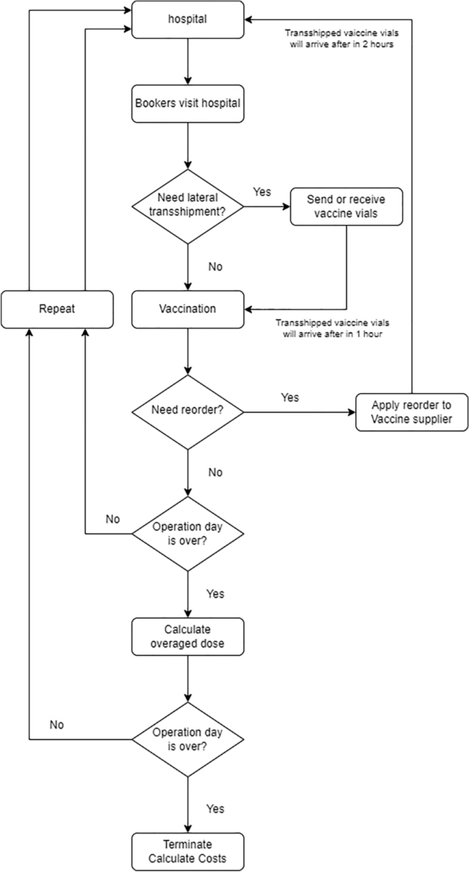
Discrete event simulation overview.
link

 Appoints Tim Cox as NMG Executive Vice President of Supply Chain")


